Cavity Scattering with Phase Noise

Cavity phase noise leads to scattering into several orthogonal temporal modes. In this example, we determine the four most populated modes of a single photon scattered on a one-sided cavity. The input pulse is in a Gaussian temporal mode with width $\tau$. The cavity has a decay rate of $\gamma$ and a dephasing rate of $\gamma_p$. This system is described in A. Kiilerich, et al., Phys. Rev. A 102, 023717 (2020).

We start by loading the packages and defining the symbolic operators and parameters.

using QuantumInputOutputusing SecondQuantizedAlgebrausing QuantumOpticsusing QuantumOpticsBase: daggerusing Plotsusing LaTeXStringsusing LinearAlgebra

# symbolic Hilbert spaceshu1 = FockSpace(:u1)hc1 = FockSpace(:c1)h = hu1 ⊗ hc1# symbolic operatorsau = Destroy(h, :a_u, 1)c = Destroy(h, :c, 2)# symbolic parameters@variables γ::Real Δ::Real γ_p::Real g_u::Number g_v::Number

We use the symbolic operators and parameters to define the SLH triples and cascade them to obtain the Hamiltonian and Lindblad for the system.

G_u = SLH(1, g_u'*au, 0) # input cavityG_c = SLH(1, √(γ)*c, Δ*c'c) # scattering cavityG_cas = ▷(G_u, G_c)

H = hamiltonian(G_cas)

(-0.5conj(g_u)*sqrt(γ))im * a_u * c' + (0.5g_u*sqrt(γ))im * a_u' * c + Δ * c' * c

L = jump_operator(G_cas)[1] # only one jump operator in this example

conj(g_u) * a_u + sqrt(γ) * c

# numerical parameters, functions and operatorsγ_ = 1.0γ_p_ = 1.5γ_Δ_ = 0.0p_sym = [γ, Δ, γ_p]p_num = [γ_, Δ_, γ_p_]dict_p = Dict(p_sym .=> p_num)# Gaussian input pulseτ = 1.0;tp = 4τu(t) = 1/(sqrt(τ)*π^(1/4)) * exp(-(t - tp)^2 / (2*τ^2))T = [0:0.002:1;]*14τΔT = T[2] - T[1]gu_ = coupling_input(u, T)dict_p_t = Dict(g_u => gu_)# numeric basesbu1 = FockBasis(1)bc1 = FockBasis(1)b = bu1 ⊗ bc1au_qo = to_numeric(au, b)c_qo = to_numeric(c, b)cdc_qo = c_qo'c_qo# translate to numeric Hamiltonian and LindbladH_QO = to_numeric(H, b; parameter = dict_p, time_parameter = dict_p_t)L_QO = to_numeric(L, b; parameter = dict_p, time_parameter = dict_p_t)

We additionally include a cavity dephasing term and solve the dynamics.

function input_output(t, ρ)    H = H_QO(t)    J = [L_QO(t), √(γ_p_)*cdc_qo]    return H, J, dagger.(J)end;# time evolutionψ0 = fockstate(bu1, 1) ⊗ fockstate(bc1, 0)t_, ρt = timeevolution.master_dynamic(T, ψ0, input_output)

We calculate the two-time autocorrelation function $g^{(1)}(t_1,t_2) = \langle L_s^\dagger(t_1) L_s(t_2) \rangle$ and diagonalize the matrix to obtain the eigenvalues with the corresponding eigenvectors. The eigenvalues correspond to the mean photon number $n_i$ in the corresponding temporal eigenvector mode $v_i$.

Ls(t) = (gu_(t))'*au_qo + √(γ_)*c_qog1_m = correlation_matrix(T, ρt, input_output, Ls);

p = heatmap(    T,    T,    real.(g1_m);    c = :inferno,    xlabel = L"\gamma t_2",    ylabel = L"\gamma t_1",    colorbar_title = L"g^{(1)}(t_1,t_2)",    size = (450, 350),)p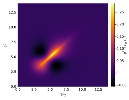

The eigenvalues and corresponding eigenvectors are sorted in ascending order, which means the last eigenvalue corresponds to the highest populated temporal mode.

F = eigen(g1_m)n_avg = round.(real.(F.values)*ΔT; digits = 2)modes = F.vectorsv_t(i) = modes[:, end-i+1] / √(ΔT)

colors = [:blue, :red, :green, :black]p = plot()for i = 1:4    plot!(p, T, real.(v_t(i)); color = colors[i], label = "n$(i)=$(n_avg[end-i+1])")endplot!(p; xlabel = "time (1/γ)", legend = :best, size = (500, 350))p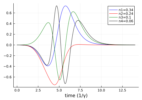

We want to note that the temporal modes and average photon numbers are different to the ones in the paper A. Kiilerich, et al., Phys. Rev. A 102, 023717 (2020) due to a typo in their numerical model.

Package versions

These results were obtained using the following versions:

using InteractiveUtilsversioninfo()using PkgPkg.status([    "QuantumInputOutput",    "SecondQuantizedAlgebra",    "QuantumOptics",    "Plots",    "LaTeXStrings",])

Julia Version 1.13.2
Commit 45b6d15e34b (2026-10-14 20:33 UTC)
Build Info:
  Official https://julialang.org release
Platform Info:
  OS: Linux (x86_64-linux-gnu)
  CPU: 4 × Intel(R) Xeon(R) Platinum 8370C CPU @ 2.80GHz
  WORD_SIZE: 64
  LLVM: libLLVM-20.1.8 (ORCJIT, icelake-server)
  GC: Built with stock GC
Threads: 1 default, 0 interactive, 1 GC (on 4 virtual cores)
Environment:
  JULIA_PKG_SERVER_REGISTRY_PREFERENCE = eager
  JULIA_DEBUG = Documenter,Literate
  JULIA_NUM_THREADS = 1
Status `~/work/QuantumInputOutput.jl/QuantumInputOutput.jl/docs/Project.toml`
  [b964fa9f] LaTeXStrings v1.4.1
  [91a5bcdd] Plots v1.41.7
  [18f9eda6] QuantumInputOutput v0.5.3 `~/work/QuantumInputOutput.jl/QuantumInputOutput.jl`
  [6e0679c1] QuantumOptics v1.2.10
⌅ [f7aa4685] SecondQuantizedAlgebra v0.11.0
Info Packages marked with ⌅ have new versions available but compatibility constraints restrict them from upgrading. To see why use `status --outdated`

This page was generated using Literate.jl.